
After looking at how a Bloom Filter works and moving on to understand a Count-Min Sketch, we were left with the final problem of identifying the most frequent reports we see at Report URI. Looking at our stream of hundreds of millions of reports per day, we're going to identify the most frequent reports quickly and easily with Top-K!

Bloom Filters and Count-Min Sketch
I have some really detailed posts on these two probabilistic data structures that are required reading before this post if you don't already know how they work. Bloom Filters are massively space efficient and can tell us if we've ever seen a particular report before or not at Report URI. I wrote a follow up blog post called When Pwned Passwords Bloom to show how you can use a Bloom Filter to query the entire Have I Been Pwned data set for Pwned Passwords locally, with less than 3GB of RAM! The limitation of the Bloom Filter was that it could only tell us if we've seen the report before or not, but not how many times we'd seen the report. That's where the Count-Min Sketch came in which could tell us how many times a particular report had been seen before with quite a good level of accuracy. I gave another demonstration of the Pwned Passwords data being used in a Count-Min Sketch in a blog post called Sketchy Pwned Passwords and that worked out pretty well too. The problem with the CMS was that it can tell you the frequency of an item that you use to query against the CMS, but it can't return a list of the Top 10 items, for example. That's where the Top-K data structure comes in!
Top-K
If you didn't read my blog posts on the Bloom Filter and Count-Min Sketch, and you don't know how they work, it would probably be advisable to read those first and then come back to this post! The Top-K data structure builds on top of the explanations given in the Bloom Filter and Count-Min Sketch posts and I will be working on the assumption of an understanding of those for my explanations here.
Just like the Bloom Filter and Count-Min Sketch, the Top-K data structure does not store all items from a set which is how it manages to remain so small, even for enormous data sets. When starting out with our explanation, we'll be starting with something that looks very similar to the last data structure we looked at in the Count-Min Sketch blog post, a 2-dimensional array as follows.
| 0 | 1 | 2 | 3 | 4 | 5 | 6 | 7 | 8 | 9 | |
|---|---|---|---|---|---|---|---|---|---|---|
| topkh1 | 0 | 0 | 0 | 0 | 0 | 0 | 0 | 0 | 0 | 0 |
| topkh2 | 0 | 0 | 0 | 0 | 0 | 0 | 0 | 0 | 0 | 0 |
| topkh3 | 0 | 0 | 0 | 0 | 0 | 0 | 0 | 0 | 0 | 0 |
As you can see we have an array of width w = 10 and depth d = 3, which has hash functions [h1, h2, ..., hd] much like we did in the Count-Min Sketch. The first difference now comes when we insert items into the Top-K where the process is a little different and we don't just insert/increment the count. Instead, we're now inserting a key:value pair of data which includes a fingerprint fp of the item and the count for the item.
topkh1[h1(a) % w = 2] = {fp(a), count}
topkh2[h2(a) % w = 7] = {fp(a), count}
topkh3[h3(a) % w = 8] = {fp(a), count}
Our array would now look like this if item a had a count of 12.
| 0 | 1 | 2 | 3 | 4 | 5 | 6 | 7 | 8 | 9 | |
|---|---|---|---|---|---|---|---|---|---|---|
| topkh1 | 0 | 0 | fp(a):12 | 0 | 0 | 0 | 0 | 0 | 0 | 0 |
| topkh2 | 0 | 0 | 0 | 0 | 0 | 0 | 0 | fp(a):12 | 0 | 0 |
| topkh3 | 0 | 0 | 0 | 0 | 0 | 0 | 0 | 0 | fp(a):12 | 0 |
Let's add a few more items, b, c and e, with counts 5, 7 and 18 to fill it a little more and set the remaining cells to null:0.
| 0 | 1 | 2 | 3 | 4 | 5 | 6 | 7 | 8 | 9 | |
|---|---|---|---|---|---|---|---|---|---|---|
| topkh1 | null:0 | fp(b):5 | fp(a):12 | null:0 | fp(e):18 | fp(c):7 | null:0 | null:0 | null:0 | null:0 |
| topkh2 | fp(c):7 | null:0 | null:0 | null:0 | null:0 | null:0 | fp(e):18 | fp(a):12 | null:0 | fp(b):5 |
| topkh3 | null:0 | fp(e):18 | null:0 | fp(c):7 | null:0 | fp(b):5 | null:0 | null:0 | fp(a):12 | null:0 |
Now if we want to insert item f with count 22, we can look in more detail at the process to add an item to the Top-K structure, because adding items is more complex than the process shown above. For any item n that we want to insert, we must do the following.
Case 1 - the count is 0:
topkhd[hd(n) % w].count == 0
then:
topkhd[hd(n) % w] = {fp(n), n.count}
Basically, if the counter in the index we're looking at is 0, then we simply insert the fingerprint and count straight into the array, job done!
Case 2 - the count is greater than 0 and fingerprint matches:
topkhd[hd(n) % w].count > 0 && topkhd[hd(n) % w].fp == fp(n)
then:
topkhd[hd(n) % w].count += n.count
If the counter in the array index we're looking at is greater than 0, and the fingerprint of the item in this index is the same as the fingerprint of the item we're adding, we simply add the count of the item we're inserting to the count in the array.
Case 3 - The count is greater than 0 and fingerprint does not match:
topkhd[hd(n) % w].count > 0 && topkhd[hd(n) % w].fp != fp(n)
then:
topkhd[hd(n) % w].count -= 1 with Pdecay probability
This is where the magic happens. If the counter in the array index we're looking at is greater than 0, and the fingerprint of the item in this index is not the same as the fingerprint of the item we're adding, we need to decay the counter in the array. The amount we decay it by is determined by the decay probability you set when you create the Top-K structure, for us decay = 0.9, raised to the power of the counter in the index already shown here as C. Here are two examples of the counter C in the index being 10 or 100,000.
Pdecay = decayC
Pdecay = 0.910
Pdecay = 0.3486784401
Pdecay = decayC
Pdecay = 0.9100,000
Pdecay = 1.78215×10-4576
For our example above of adding item f with count 22, we would repeat the decay process 22 (f.count) times. The probability that we'd decay the counter in the existing array index is drastically different depending on how large the existing counter in the index is.
If the existing counter in the array is huge, and we have a low count like 22 for item f that we're trying to insert, the chance of us decaying the existing counter is minimal.
If the existing counter in the array is small, the chance of us decaying the existing counter is considerable and we will quickly reduce it.
Finally, and most importantly, if we decay the existing counter in the array to 0, the fingerprint for the existing item in the array is removed and the fingerprint for the new item n we're inserting is inserted along with the remaining count. The existing item is removed from the Top-K data structure and the new item n is inserted.
HeavyKeeper
The process described above is known as HeavyKeeper and is the basis for how Top-K works in Redis. If you have a small selection of items with a very large count, the chances of their counts being decayed by even millions of items with a low count is minimal because as the counter in the array increases, the chance of decay decreases. This is known as the exponentially-weakening decay probability and it favours elephant flows over mouse flows.
I introduced the terms elephant flow and mouse flow in the previous blog post on Count-Min Sketch, but they basically refers to items with a large count (elephant flow) and a small count (mouse flow). The HeavyKeeper method favours elephant flows as once they are established in the Top-K data structure, it becomes increasingly hard to decay them back out. Even with a substantial volume of mouse flows, they will not be able to decay an elephant flow out of the Top-K, only another elephant flow could do that. This is why the HeavyKeeper is named as it is, because it keeps elephant flows, and how it does so.
Min-Heap Binary Tree
The final step of the process is that the implementation of Top-K maintains a min-heap binary tree containing all of the Top-K elephant flows, allowing for fast and reliable retrieval of the list of Top-K items.
A min-heap is a simple binary tree where the value in a node is less than or equal to children of that node. Here's a simple example with 10 nodes that would be used if k = 10.
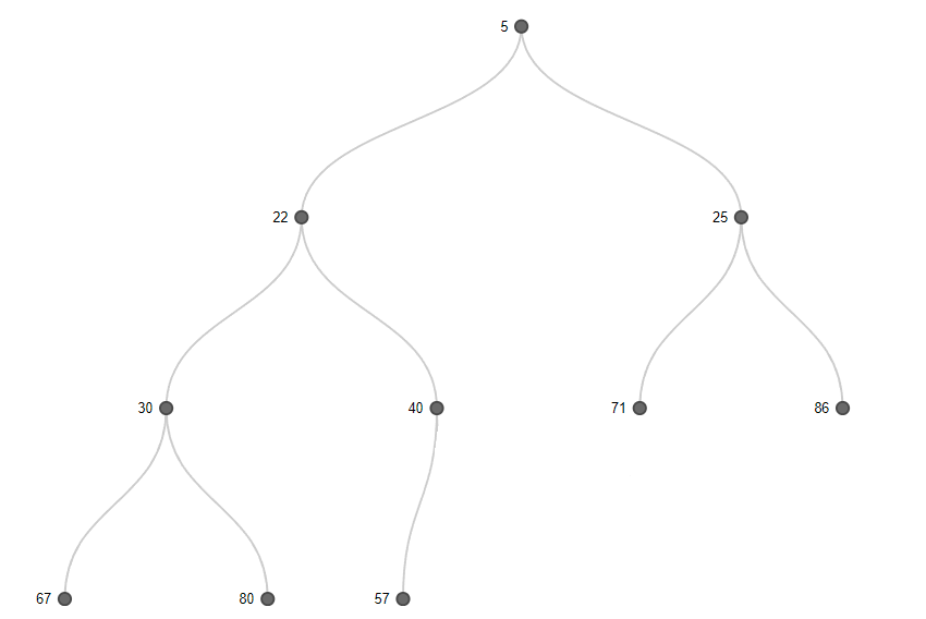
A min-heap can also be represented as a 2-dimensional array like this.
| 0 | 1 | 2 | 3 | 4 | 5 | 6 | 7 | 8 | 9 | |
|---|---|---|---|---|---|---|---|---|---|---|
| min-heap | 5 | 22 | 25 | 30 | 40 | 71 | 86 | 67 | 80 | 57 |
In our min-heap, the node would hold the fingerprint of the item, the count for the item and the item itself for all k items in the Top-K list. For simplicity and space concerns in my tables below, I'm only showing the fingerprint and the count, so just remember that the item itself is in there too!
| 0 | 1 | 2 | 3 | 4 | 5 | 6 | 7 | 8 | 9 | |
|---|---|---|---|---|---|---|---|---|---|---|
| min-heap | fp(a):5 | fp(s):22 | fp(j):25 | fp(q):30 | fp(v):40 | fp(l):71 | fp(p):86 | fp(d):67 | fp(k):80 | fp(h):57 |
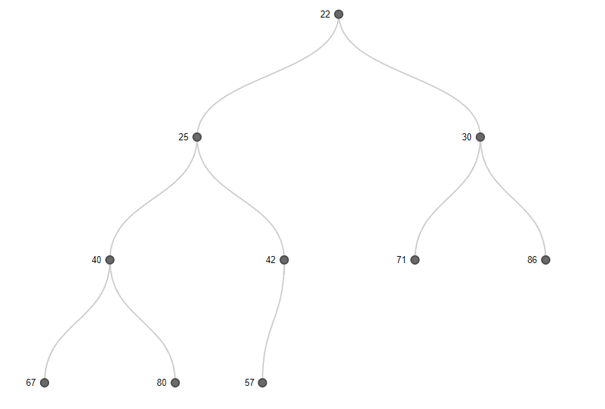
After adding an item n to the HeavyKeeper structure above you would have the new count for that item. You would then take the new count for item n and query the min-heap to see if the count is larger than the smallest item in the heap, which is the first item in the array. If the new count for item n is larger than the smallest item in the min-heap, we have a new contender to enter the min-heap, and thus the Top-K. The first step is to search the heap and identify if item n is already present and if it is, update the count. If we were inserting item v into the heap, which is already present, we'd simply update the count for the existing item and re-heapify down from the current index. Let's say item n has a count of 42. We can easily determine that 42 is larger than 5, so it needs to go into the min-heap, and we can also see that item n is not already in the heap to update the count. We would then remove the root node of the tree and insert our new item.
| 0 | 1 | 2 | 3 | 4 | 5 | 6 | 7 | 8 | 9 | |
|---|---|---|---|---|---|---|---|---|---|---|
| min-heap | fp(n):42 | fp(s):22 | fp(j):25 | fp(q):30 | fp(v):40 | fp(l):71 | fp(p):86 | fp(d):67 | fp(k):80 | fp(h):57 |
To then re-order, we simply swap the item n with the item to the right if the count to the right is smaller than 42. Here we can see the four steps:
| 0 | 1 | 2 | 3 | 4 | 5 | 6 | 7 | 8 | 9 | |
|---|---|---|---|---|---|---|---|---|---|---|
| min-heap | fp(s):22 | fp(n):42 | fp(j):25 | fp(q):30 | fp(v):40 | fp(l):71 | fp(p):86 | fp(d):67 | fp(k):80 | fp(h):57 |
| 0 | 1 | 2 | 3 | 4 | 5 | 6 | 7 | 8 | 9 | |
|---|---|---|---|---|---|---|---|---|---|---|
| min-heap | fp(s):22 | fp(j):25 | fp(n):42 | fp(q):30 | fp(v):40 | fp(l):71 | fp(p):86 | fp(d):67 | fp(k):80 | fp(h):57 |
| 0 | 1 | 2 | 3 | 4 | 5 | 6 | 7 | 8 | 9 | |
|---|---|---|---|---|---|---|---|---|---|---|
| min-heap | fp(s):22 | fp(j):25 | fp(q):30 | fp(n):42 | fp(v):40 | fp(l):71 | fp(p):86 | fp(d):67 | fp(k):80 | fp(h):57 |
| 0 | 1 | 2 | 3 | 4 | 5 | 6 | 7 | 8 | 9 | |
|---|---|---|---|---|---|---|---|---|---|---|
| min-heap | fp(s):22 | fp(j):25 | fp(q):30 | fp(v):40 | fp(n):42 | fp(l):71 | fp(p):86 | fp(d):67 | fp(k):80 | fp(h):57 |
This gives us our newly ordered min-heap!
Using Top-K at Report URI
I've already talked about Bloom Filters and Count-Min Sketch, along with how we plan to use them at Report URI, but Top-K is the first probabilistic data structure that I've blogged about that is already deployed in production for use at Report URI and not just being tested.
Every week the team at Report URI receive an email with the most frequently blocked reports from the last 7 days. This allows us to spot new trends in terms of what's being blocked, perhaps a customer has a misconfiguration and we can reach out to them or a browser extension has gone rogue and is loading an asset that causes a huge amount of CSP reports. This data is also always available on an ongoing basis and helps us in our work to refine filters, spot new threats, support customers and much more.
We use our dedicated Redis cache for handling reports and report-based data to store the Top-K data structure and for now, we're tracking the Top 100 most common blocked items via CSP.
10.138.132.251:6379> TOPK.INFO THREATS_TOPK
1) k
2) (integer) 100
3) width
4) (integer) 8
5) depth
6) (integer) 7
7) decay
8) "0.90000000000000002"
The Top-K data structure takes up basically no memory!
10.138.132.251:6379> DEBUG OBJECT THREATS_TOPK
Value at:0x7f1e9a415050 refcount:1 encoding:raw serializedlength:4347 lru:10482554 lru_seconds_idle:11
Determining Dimensions
We originally started out with the default dimensions provided by RedisBloom but found that they weren't favourable to our setup. I've also done some extensive testing of Top-K with the Pwned Passwords data set, as I did with When Pwned Password Bloom and Sketchy Pwned Passwords for the Bloom Filter and Count-Min Sketch respectively, but we're still experimenting.
After reading a lot of articles and papers on Top-K/Heavy Keeper and related data structures ([1][2][3][4][5] et al.), it would seem there is no clear-cut, single answer for the question 'What are the correct dimensions?'. From those articles and papers the best I've managed to come up with so far is:
width = k * log(k)
depth = max(5, log(k))
Still though, even when testing this with production data, I'm still convinced that there is some tweaking that needs to be done on these dimensions and that a lower depth seems to yield better results (higher accuracy) in most cases. For now, our plan is to continue to refining the dimensions over time and I'm hoping to publish my testing with the Pwned Passwords data too!