
Have we seen this report before? It sounds like a simple question to ask of a service that collects and processes hundreds of millions of reports per day, and in many ways it is, but in some ways it isn't. Here's how a probabilistic data structure called a Bloom Filter can make it surprisingly easy to answer that question!

Our data volume
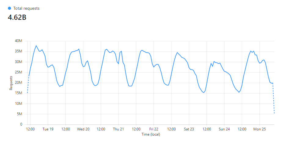
In The first 3 months of report-uri.io, we were processing in the region of 250,000 reports per week. Not bad for a service that was just starting out, but things continued to grow. Just a few years later I wrote Report URI: A week in numbers and we processing over 2,600,000,000 reports per week! Understandably, our infrastructure has gone through quite a lot of changes in that time and so have the approaches we take to handling and working with that much data. Looking at our live data today from our Cloudflare dashboard, in the last week we did just over 4,620,000,000 reports... That's pretty wild!
As the amount of data we handle continues to increase, we face more and more challenges with handling and processing it. Things that were once simple become less so as you scale and new ways of solving problems are required.
Threat Intelligence
Internally, we have some data gathering and analysis that we do on report data to try and improve our service for our customers. For example, one of our most important features is filtering CSP reports that aren't useful. These can be triggered by software on the client, a dodgy browser extension screwing with the page or the user being behind a proxy that's messing stuff up. Either way, reports can be triggered that a site operator just doesn't need to know about and we do our best to filter those out.
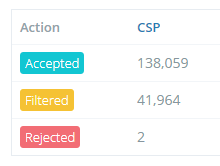
Looking at that overview of my report numbers, which is available to all Report URI users on their account homepage, you can see that our service has filtered almost 25% of my inbound reports! That's a lot of stuff that I don't need to worry about looking at, but identifying which reports to filter can be quite difficult.
When investigating a new candidate for filtering, we want to be absolutely sure that it's safe to filter and won't cause any problems for any user if we filter it. Because of the high bar we set here, you can see noisy reports making it into your account for a short period while they're reviewed and identified, because it's better to be safe than sorry. One of the things that really helps in our analysis of reports like this is the volume that the report is being sent in. Are we seeing only one of these reports a week or are we seeing a thousand of them a second? Looking at the frequency of reports like this is useful for filtering, and a few more features we're yet to talk about, but it can be tricky to monitor. Another great metric to look at is if we've even seen this particular report before at all because if it's the first time we've ever seen a report, it probably warrants some further inspection.
That's a whole lot of data
Another problem that we face is that we only keep historic report data for 90 days, after which the raw report data is purged and counts/metrics are retained to populate graphs and statistics beyond the last 90 days. Despite our best efforts in keeping this data to a minimum, normalising reports and having a strict data retention policy, we still have 3.27TB of data on disk at the time of writing, and querying against that amount of data is no small task. Our retention policy also makes it basically impossible to answer the question 'have we seen this report before?' because we don't keep all historic reports to query against.
I've talked a lot about our data storage mechanism, Azure Table Storage, in the past in a few different blog posts, and despite the fact that it's not built for queries like the ones we'd need to run here, even if it were, consistently running many queries against such a large dataset, that continues to grow, seems like a bad idea. We also have no option to keep all historic reports either, but even then it's not only the size of the dataset that's the problem either. At our peak times we can be processing almost 14,000 inbound CSP reports per second! If we want to query the database to see if we've seen this report before or retrieve the count of how many times we've seen this report, or just about anything else we might like to query, that's a lot of additional activity.
Probabilistic Data Structures
You can do some outrageously cool things with probabilistic data structures, which sacrifice a small amount of accuracy for unbelievable space efficiency and time efficiency. I've talked about Bloom Filters before when talking about CRLite and revocation, but I didn't cover them in the depth that I'd like to and how we might use them at Report URI. After talking about Bloom Filters in this post, I'll also be talking about other probabilistic data structures like Count-Min Sketch and Top-K that can do even more cool things in following posts, so stay tuned.
Bloom Filters
The basic operation of a Bloom Filter is relatively simple but there are some things to consider when creating them and using them. The main benefit of a Bloom Filter is that they can allow you to check if an item is a member of a set of items without having to store the entire set of items. This is where they get their awesome space efficiency from. In our case, we're going to be checking if an incoming CSP report (the item) has been seen before in all CSP reports we've ever processed (the set of items).
Given that our last 90 days of reports comes in at close to 4TB, I'd dread to think how much data we'd have if we kept all historic reports, it'd be in the tens of TBs quite easily. Storing that amount of data and querying against it would be a huge burden, but using a Bloom Filter we're only going to need a few GB of RAM and a few microseconds to perform the query!
How they work
To get started, we're going to look at this simple Bloom Filter, which is just an array of bits called bloom, all initialised to a value of 0, of size m where m = 10 for my array.
| 0 | 1 | 2 | 3 | 4 | 5 | 6 | 7 | 8 | 9 | |
|---|---|---|---|---|---|---|---|---|---|---|
| bloom | 0 | 0 | 0 | 0 | 0 | 0 | 0 | 0 | 0 | 0 |
In order to add an item a to the filter, where item a is a CSP report we've processed, we need to hash the item to figure out which bits to set in the array. We will have k hash functions to use and I'm going to use two hash functions in this example so k = 2 giving me hash functions h1 and h2, [h1, h2, ..., hk].
To add item a to the filter, which is an item from the set of n items (all CSP reports added to the filter), we need to set the bits at k locations. We hash item a with each hash function to produce the index in the bloom array where we're going to set the bits as follows:
bloom[h1(a) % m] = 1
bloom[h2(a) % m] = 1
Assuming that h1(a) % m = 2 and h2(a) % m = 5, we would do the following:
bloom[2] = 1
bloom[5] = 1
That means our array would now look like this:
| 0 | 1 | 2 | 3 | 4 | 5 | 6 | 7 | 8 | 9 | |
|---|---|---|---|---|---|---|---|---|---|---|
| bloom | 0 | 0 | 1 | 0 | 0 | 1 | 0 | 0 | 0 | 0 |
To now add another CSP report, item b, to the filter, we need to set the bits at the following locations:
bloom[h1(b) % m] = 1
bloom[h2(b) % m] = 1
Assuming that h1(b) % m = 5 and h2(b) % m = 8, we would do the following:
bloom[5] = 1
bloom[8] = 1
Our array would now look like this:
| 0 | 1 | 2 | 3 | 4 | 5 | 6 | 7 | 8 | 9 | |
|---|---|---|---|---|---|---|---|---|---|---|
| bloom | 0 | 0 | 1 | 0 | 0 | 1 | 0 | 0 | 1 | 0 |
We've now inserted two items into the filter, item a and item b, and we can perform a query against the filter if we'd like to. In order to query if an item is present in the filter, you have to hash the item and lookup the values of the bits at the appropriate locations. Let's say we want to query for the presence of item c, which is an incoming CSP report, we'd look at the following locations in the array:
bloom[h1(c) % m = 4] == 0
bloom[h2(c) % m = 9] == 0
Because the two values at bloom[4] and bloom[9] are 0, we can say that item c is definitely not in the set n, meaning we've never seen this CSP report before. Let's try to query item d from our filter which is another inbound CSP report.
bloom[h1(d) % m = 3] == 0
bloom[h2(d) % m = 5] == 1
Here we can see something called a hash collision has occurred because h2(d) % m = h1(b) % m = 5. The bit located at bloom[5] was set for item b but has now shown up in the query for item d which is not present in the filter. Still though, bloom[3] == 0 so we can say that item d is definitely not in the set n or this bit would have been set.
The problem we might encounter comes when we try to query item e from the filter.
bloom[h1(e) % m = 2] == 1
bloom[h2(e) % m = 8] == 1
Now we've had two hash collisions occurr because h1(a) % m = h1(e) % m = 2 and h2(b) % m = h2(e) % m = 8. When we query a Bloom Filter and all bits are set for the item in the query, we can say that the item was possibly present in the data set n because hash collisions can make it appear as if it was present, even though it wasn't. This is the 'probabilistic' nature of Bloom Filters, they can only tell us one of two things:
- The item is definitely not in the set n.
- The item is probably in the set n.
Of course the same is also true for item a which we did insert into the filter, but we can only say it is probably in the set because when we query the filter we get the following:
bloom[h1(a) % m = 2] == 1
bloom[h2(a) % m = 5] == 1
These bits could have been set because item a is present in the set n, or, because of collisions created by adding other items.
In order to keep the Bloom Filter updated with all CSP reports we've ever processed, all you have to do is query to see if the CSP report is present in the filter, and if it isn't present, then you set the appropriate bits in the array so that the next time you see the report and query the filter, it will indicate that we've seen the report before.
Avoiding Collisions
You can control how likely collisions are in your Bloom Filter and this will allow you to control the probability of a false positive. The three values under your control are:
m = the size of the array
n = how many items will be placed in the filter
k = how many hash functions you use
By making the size of the array m larger, you reduce the chance of a false positive, but increase the memory requirements of the filter. The chance of a false positive reduces because as the width of the array increases, the chance of a hash collision decreases, but this larger array will cost you storage space.
By reducing the number of items n that will be placed in the array you can also reduce collisions because with less items in the filter, there is less chance that their hashes will collide for an array of any given size.
To some extent, you can also increase the number of hash functions k that you use to reduce the chance of a false positive caused by collisions. If each hash function is pairwise independent, meaning that none of the hash functions will ever produce the same index for the same item, you then need to suffer k collisions for there to be a false positive. This method will, however, quickly bring diminishing returns and then become a detriment due to overpopulating the array and causing more collisions. A great example is consider our array of size m = 10 and assume we had k = 10 hash functions. Once the first item was set in the filter, everything would be a false positive after that because all bits in the array are set.
The main consideration is that m and k must be decided when creating the Bloom Filter and can't be changed at a later stage, and you need a reasonable idea for the value of n at the time of creating the filter too. Fortunately, there are some great Bloom Filter Calculators ([1][2]) that make figuring out the required values much easier!
n = ceil(m / (-k / log(1 - exp(log(p) / k))))
p = pow(1 - exp(-k / (m / n)), k)
m = ceil((n * log(p)) / log(1 / pow(2, log(2))));
k = round((m / n) * log(2));
If we'd like to put all of our reports from Report URI into a filter, then n = ~700,000,000,000, and we'd like to query with a false positive probability p = 0.01 (1%), then we'd need a filter of size m = 6709540864158!
m = ceil((n * log(p)) / log(1 / pow(2, log(2))));
m = ceil((700000000000 * log(0.01)) / log(1 / pow(2, log(2))));
m = 6709540864158;
That's ~840GB... This is of course assuming that every report is unique though, which they're not. Based on our anecdotal data, the majority of reports are actually duplicates of previously seen reports, but the Bloom Filter is exactly the mechanism to help us determine this with more accuracy. By placing all reports in the filter we can quickly query it to see if we've probably seen a report before and take action on only new reports we're seeing for the first time. We still need to come up with a value to start out though, so let's take a wild guess and say that we've seen each report, on average, one hundred times, meaning that n = 7,000,000,000. This makes things a lot better.
m = ceil((n * log(p)) / log(1 / pow(2, log(2))));
m = ceil((7000000000 * log(0.01)) / log(1 / pow(2, log(2))));
m = 67095408642;
Our filter is now only ~8.4GB in size (840/100) because Bloom Filters exhibit a linear space complexity O(m) and we kept p constant whilst reducing n. That's quite a small amount of memory to store the Bloom Filter and it would allow us to query against it for every single inbound report to see if we've ever seen that report before without touching our database and it would include previous reports that have since been purged from disk as they will still be present in the filter, assuming we maintain it on an ongoing basis.
Putting Bloom Filters to use
Bloom Filters are the basic element of other more complex probabilistic data structures we're also going to be using at Report URI very soon, like Count-Min Sketch and Top-K, but they depend upon the basic operation and understanding of a Bloom Filter to be able to use them. That said, we are considering using a global Bloom Filter to identify unique reports on their way into our service and we're also considering the use of Bloom Filters on a per account/team basis to replace our current mechanism for identifying new reports that we alert you to.
Other common uses for Bloom Filters are wide ranging but there are some good examples in the security space. Checking weak passwords against a large dataset is one possible option where an enormous amount of passwords can be queried against quickly to rule out bad passwords. Google Safe Browsing also uses a Bloom filter to query for malicious URLs, allowing you to quickly determine that a URL is not malicious or call back to the service for confirmation if the URL flags as possibly malicious in the Bloom Filter. It's also common to see Bloom Filters used in caching to avoid "one-hit-wonders", where an asset is only requested once and doesn't need caching. The Bloom Filter can answer the question 'have we seen this request before?' and if you have, then you cache the item, but if you haven't, you can avoid caching it. This means items will only get cached on the second time they are requested and avoids the cache being overpopulated with items that are not regularly requested.
Low Cost
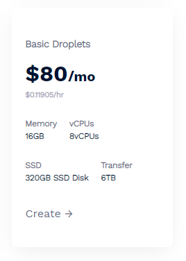
Our hosting provider, DigitalOcean, has a VPS that can comfortably handle the above example Bloom Filter task for only $80/mo which makes this quite a reasonable cost for such a powerful feature.
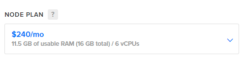
The referral link above will also get you $100 in credit so you could play around with this for a whole month with no cost! If you don't want to setup and manage your own Redis instance then you can use a managed solution that comes in at $240/mo instead.
Note that you need to check for support of the redisbloom module which allows for the use of features like Bloom Filters and the other probabilistic data structures I will be discussing, but it's easy to get started!
Limitations of a Bloom Filter
The ability to so quickly and easily determine if we've ever seen a report before would be mega-useful in our report ingestion pipeline, especially because we don't need to store all historic reports and query over them, but I'd love to go one step further and also know how many times we've seen a report before too. A Bloom Filter simply can't do that, but in my next blog post on probabilistic data structures I'll be looking at how we can answer that question with something called a Count-Min Sketch.
Alongside that I'm also working on a very real demonstration of just how practical a Bloom Filter can be with a real-world example that I'm sure most people will find to be quite an interesting read so stay tuned for that!